Advanced filtering
To filter using search:
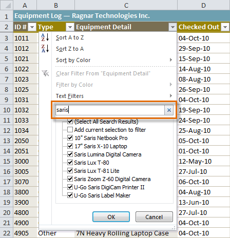
Searching for data is a convenient alternative to checking or unchecking data from the list. You can search for data that contains an exact phrase, number, date, or simple fragment. For example, searching for the exact phrase Saris X-10 Laptop will display only Saris X-10 laptops. Searching for the word Saris, however, will display Saris X-10 laptops and any other Saris equipment, including projectors and digital cameras.
- 1- From the Data tab, click the Filter command.
- 2- Click the drop-down arrow in the column you want to filter. In this example, we'll filter the Equipment Detail column to view only a specific brand.
- 3- Enter the data you want to view in the Search box. We'll enter the word Saris to find all Saris brand equipment. The search results will appear automatically.
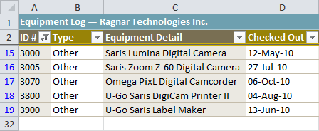
- 4- Check the boxes next to the data you want to display. We'll display all of the data that includes the brand name Saris.
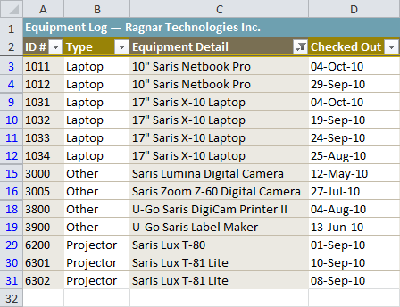
- 5- Click OK. The worksheet will be filtered according to your search term.
Using advanced text filters
Advanced text filters can be used to display more specific information, such as cells that contain a certain number of characters or data that does not contain a word you specify. In this example, we'll use advanced text filters to hide any equipment that is related to cameras, including digital cameras and camcorders.
- 1- From the Data tab, click the Filter command.
- 2- Click the drop-down arrow in the column of text you want to filter. In this example, we'll filter the Equipment Detail column to view only certain types of equipment.
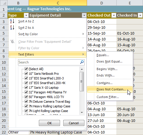
- 3- Choose Text Filters to open the advanced filtering menu.
- 4- Choose a filter. In this example, we will choose Does Not Contain to view data that does not contain the text we specify.
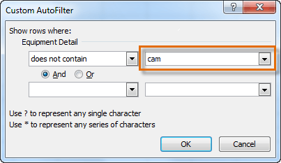
- 5- The Custom AutoFilter dialog box appears.
- 6- Enter your text to the right of your filter. In this example, we'll enter cam to view data that does not contain these letters. That will exclude any equipment related to cameras, such as digital cameras, camcorders, camera bags, and the digicam printer.
- 7- Click OK. The data will be filtered according to the filter you chose and the text you specified.
Using advanced date filters
Advanced date filters can be used to view information from a certain time period, such as last year, next quarter, or between two dates. Excel automatically knows your current date and time, making this tool easy to use. In this example, we'll use advanced date filters to view only the equipment that has been checked out this week.
- 1- From the Data tab, click the Filter command.
- 2- Click the drop-down arrow in the column of dates you want to filter. In this example, we'll filter the Checked Out column to view only a certain range of dates.
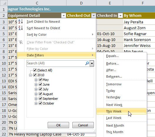
- 3- Choose Date Filters to open the advanced filtering menu.
- 4- Click a filter. We'll choose This Week to view equipment that has been checked out this week.
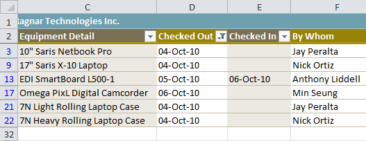
- 5- The worksheet will be filtered according to the date filter you chose.
If you're working along with the example file, your results will be different from the images above. If you want, you can change some of the dates so the filter will give more results.
Using advanced number filters
Advanced number filters allow you to manipulate numbered data in different ways. For example, in a worksheet of exam grades you could display the top and bottom numbers to view the highest and lowest scores. In this example, we'll display only certain types of equipment based on the range of ID #s that have been assigned to them.
- 1- From the Data tab, click the Filter command.
- 2- Click the drop-down arrow in the column of numbers you want to filter. In this example, we'll filter the ID # column to view only a certain range of ID #s.
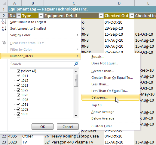
- 3- Choose Number Filters to open the advanced filtering menu.
- 4- Choose a filter. In this example, we'll choose Between to view ID #s between the numbers we specify.
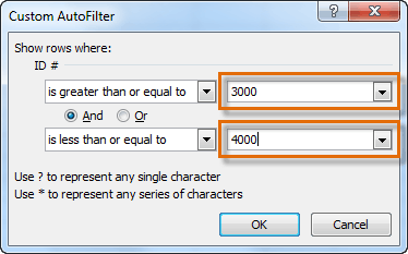
- 5- Enter a number to the right of each filter. In this example, we'll view ID #s greater than or equal to 3000 but less than or equal to 4000. This will display ID #s in the 3000-4000 range.
- 6- Click OK. The data will be filtered according to the filter you chose and the numbers you specified.


Comments
Post a Comment