Filtering data
Filters can be applied in different ways to improve the performance of your worksheet. You can filter text, dates, and numbers. You can even use more than one filter to further narrow your results.
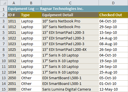
- 1- Begin with a worksheet that identifies each column using a header row.
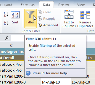
- 2- Select the Data tab, then locate the Sort & Filter group.
- 3- Click the Filter command.
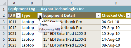
- 4- Drop-down arrows will appear in the header of each column.
- 5- Click the drop-down arrow for the column you want to filter. In this example, we'll filter the Type column to view only certain types of equipment.
- 6- The Filter menu appears.
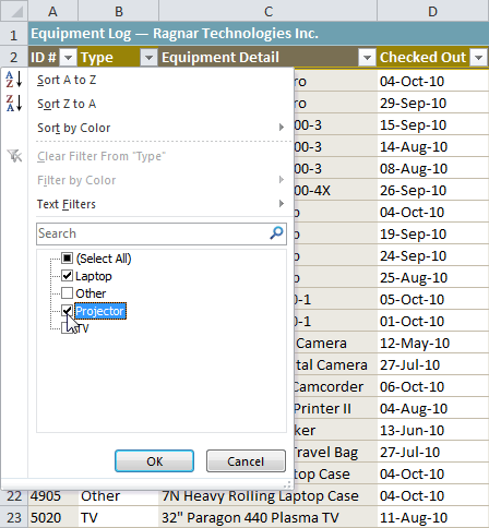
- 7- Uncheck the boxes next to the data you don't want to view, or uncheck the box next to Select All to quickly uncheck all.
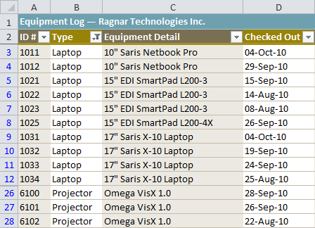
- 8- Check the boxes next to the data you do want to view. In this example, we'll check Laptop and Projector to view only these types of equipment.
- 9- Click OK. All other data will be filtered, or temporarily hidden. Only laptops and projectors will be visible.
Filtering options can also be found on the Home tab, condensed into the Sort & Filter command.
To add another filter:
Filters are additive, meaning you can use as many as you need to narrow your results. In this example, we'll work with a spreadsheet that has already been filtered to display only laptops and projectors. Now we'll display only laptops and projectors that were checked out during the month of August.
- 1- Click the drop-down arrow where you want to add a filter. In this example, we'll add a filter to the Checked Out column to view information by date.
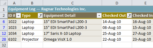
- 2- Uncheck the boxes next to the data you don't want to view. Check the boxes next to the data you do want to view. In this example, we'll check the box next to August.
- 3- Click OK. In addition to the original filter, the new filter will be applied. The worksheet will be narrowed down even further.
To clear a filter:
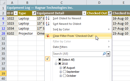
- 1- Click the drop-down arrow in the column from which you want to clear the filter.
- 2- Choose Clear Filter From.
- 3- The filter will be cleared from the column. The data that was previously hidden will be on display once again.
- To instantly clear all filters from your worksheet, click the Filter command on the Data tab.


Comments
Post a Comment